Ambient Occlusion

Special thanks to Mikael Hvidtfeldt Christensen for his "naive ambient occlusion" algorythm (http://blog.hvidtfeldts.net/). The effect is cool and gives the raytracer a cartoon-like style that I really like.

Extreme Interactive Raytracing

Those who know about raytracing will understand my excitement :) Just consider that every pixel is a ray of light that interacts with every single sphere in the 3D scene. The amout of computation is unbeleivable but this is what we get from a $300 graphics card. Feel the power and enjoy unlimited possibilities.

Cloud Ready Photorealistic Protein Visualizer / Raytracing

Download the Windows and Linux x64 / Cuda version

New video teaser detailing some of the application features

 

- nVidia 3DVision ready (Not working live yet but working hard on it!!). If you have the 3DVision Kit, download the following video and try it out!

 

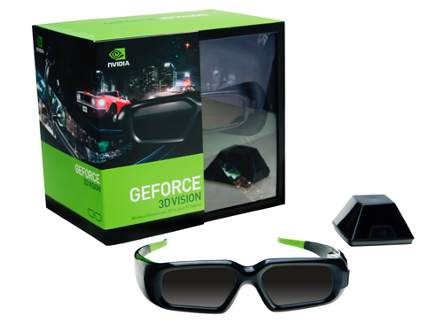
- Supports Kinect as a way to adapt visualization to the viewer.

- Cloud Ready

BVH allowing massive number of objects

 

Comparing dates with OpenCL - And a mktime function that scales

I recently came across a simple problem in C++, but a difficult one in OpenCL: comparing dates. Since I needed this functionality in one of my algorithms, I decided to implement my own OpenCL diffDays function and here is what it looks like the one bellow.

OpenCL

// Globals

__constant int DaysInMonths[12] = { 31, 28, 31, 30, 31, 30, 31, 31, 30, 31, 30, 31 };

// Macros

#define isleap(y) ((((y) % 4) == 0 && ((y) % 100) != 0) || ((y) % 400) == 0)

typedef struct

{

       int tm_sec;

       int tm_min;

       int tm_hour;

       int tm_mday;

       int tm_mon;

       int tm_year;

       int tm_wday;

       int tm_yday;

       int tm_isdst;

} TimeStructure;

void computeYearDay( TimeStructure* t )

{

       int nbDays = 0;

       for( int i=0; i<(*t).tm_mon-1; ++i )

       {

             nbDays += DaysInMonths[i];

       }

       nbDays += (*t).tm_mday;

       nbDays += isleap((*t).tm_year ) ? 1 : 0; // leap years

       (*t).tm_yday = nbDays;

}

int diffDays(TimeStructure fromDate, TimeStructure toDate)

{

       int fndays        = 0;

       float fndaysFrom = 0.f;

       float fndaysTo   = 0.f;

       int ndays = 0;

       computeYearDay(&fromDate);

       computeYearDay(&toDate);

       int toYear   = 1900 + toDate.tm_year;

       int fromYear = 1900 + fromDate.tm_year;

       fndaysFrom =  (float)(fromDate.tm_mday);

       fndaysFrom += (float)(fromDate.tm_hour)/24.f;

       fndaysFrom += (float)(fromDate.tm_min)/1440.f;

       fndaysFrom += (float)(fromDate.tm_sec)/86400.f;

       fndaysTo  = (float)(toDate.tm_mday);

       fndaysTo += (float)(toDate.tm_hour)/24.f;

       fndaysTo += (float)(toDate.tm_min)/1440.f;

       fndaysTo += (float)(toDate.tm_sec)/86400.f;

       for(int i=fromYear; i < toYear; i++) {

             ndays += isleap(i) ? 366 : 365;

       }

       fndays = ndays + (fndaysTo - fndaysFrom);

       return -fndays;

}

The funny thing about it that when I tried to compare the results between CPU execution (using OpenMP) and the OpenCL implementation, I realized that my C++ code could not scale properly. Even worse, it was slowing down as I was increasing the number of cores. After a good profiling session using Intel Parallel Studio, I realized that the slowing bit was in the mktime function provided with Microsoft Visual C++ 2010. So I ported the OpenCL function back to C++ and that resulted in an amazing x20 increase in performance on 8 CPUs. 

And I now have a mktime that scales on multicore architectures !!

C/C++

#define isleap(y) ((((y) % 4) == 0 && ((y) % 100) != 0) || ((y) % 400) == 0)

const int DaysInMonths[12] = { 31, 28, 31, 30, 31, 30, 31, 31, 30, 31, 30, 31 };

void computeYearDay( tm& t )

{

       int nbDays = 0;

       for( int i=0; i<t.tm_mon-1; ++i )

       {

             nbDays += DaysInMonths[i];

       }

       nbDays += t.tm_mday;

       nbDays += isleap(t.tm_year ) ? 1 : 0;

       t.tm_yday = nbDays;

}

int diffDays(tm b, tm a)

{

       int fndays       = 0;

       float fndaysFrom = 0.f;

       float fndaysTo   = 0.f;

       int ndays = 0;

       computeYearDay(b);

       computeYearDay(a);

       int toYear   = 1900 + a.tm_year;

       int fromYear = 1900 + b.tm_year;

       fndaysFrom  = static_cast<float>(b.tm_mday);

       fndaysFrom += static_cast<float>(b.tm_hour)/24.f;

       fndaysFrom += static_cast<float>(b.tm_min)/1440.f;

       fndaysFrom += static_cast<float>(b.tm_sec)/86400.f;

       fndaysTo  = static_cast<float>(a.tm_mday);

       fndaysTo += static_cast<float>(a.tm_hour)/24.f;

       fndaysTo += static_cast<float>(a.tm_min)/1440.f;

       fndaysTo += static_cast<float>(a.tm_sec)/86400.f;

       for(int i=fromYear; i < toYear; i++) {

             ndays += isleap(i) ? 366 : 365;

       }

       fndays = ndays + (fndaysTo - fndaysFrom);

       return -fndays;

}

Optimizing performance when using atomic operations

Here is the problem: We have a list of containers, each of them containing a variable number of floats. What we want to achieve is counting the number of containers for which the sum of float values is greater than a given limit.

The parallelism is done at a container level, meaning that each thread will process a container. The algorithm per thread is simple: walk through the list of floats and sum them up. Once this is done, there is a concurrency issue when it comes to counting the number of containers with a sum that is greater than our given limit. The simple solution is to use an atomic add in each thread when the limit condition is true. But cannot we be a bit more efficient? Of course we can!

On GPUs, threads are organized by blocks, and memory can be easily and efficiently shared between threads from the same block. So the idea is to use the atomic add at a block level rather than at a thread one. To do so, a shared 2D array is instanciated for a given 2D block so that each thread from the block has its own item in the array. By doing so, we avoid concurrency between threads from the same block.

__shared__ int r[BLOCK_SIZE][BLOCK_SIZE];

Each thread from the block can now perform its algorithm and store its result in the shared array.

// Compute the index

int x = (blockDim.x*blockIdx.x + threadIdx.x);

int y = (blockDim.y*blockIdx.y + threadIdx.y);
int index = y*(blockDim.x*blockIdx.x) + x;

      

// Here comes the Business stuff

Constainer p = containers[index];

int i = 0;

float sum = 0;

for( i = 0; i<p.nbElements; ++i )

{

  sum += p.elements[i];

}

r[threadIdx.x][threadIdx.y] = ( sum > limit ) ? 1 : 0;

Once the block of threads is done and synchronized using the __syncthreads() cuda function, the elements from the array are summed up and the result is stored in the global counter, using an atomic add. Note that this process should only be performed by one single thread from the block.

if( threadIdx.x == 0 && threadIdx.y == 0 )  // Only one thread should do this job.

{

  int s = 0;

  for( int x=0; x<BLOCK_SIZE; ++x )

  {

    for( int y=0; y<BLOCK_SIZE; ++y )

    {

      s += r[x][y];

    }

  }

  atomicAdd(result,s);

}

The full code will look like this:

struct Container

{

   int nbElements;

   float elements[NB_MAX_ELEMENTS_PER_CONTAINER];

};

__global__ void cuda_kernel( Container* containers, int* result, float limit )

{

   __shared__ int r[BLOCK_SIZE][BLOCK_SIZE];

  // Compute the index

  int x = (blockDim.x*blockIdx.x + threadIdx.x);

  int y = (blockDim.y*blockIdx.y + threadIdx.y);
  int index = y*(blockDim.x*blockIdx.x) + x;

  // Here comes the Business stuff

  Constainer p = containers[index];

  int i = 0;

  float sum = 0;

  for( i = 0; i<p.nbElements; ++i )

  {

    sum += p.elements[i];

  }

  r[threadIdx.x][threadIdx.y] = ( sum > limit ) ? 1 : 0;

  __syncthreads();

  if( threadIdx.x == 0 && threadIdx.y == 0 )

  {

    int s = 0;

    for( int x=0; x<BLOCK_SIZE; ++x )

    {

      for( int y=0; y<BLOCK_SIZE; ++y )

      {

        s += r[x][y];

      }

    }

    atomicAdd(result,s);

  }

}

extern "C" void cuda_runKernel( unsigned int nbContainers, float limit )

{

  // Run the Kernel

  dim3 block(BLOCK_SIZE,BLOCK_SIZE,1);

  int  grid = nbContainers/(block.x*block.y);

  cuda_kernel<<<grid,block>>>( d_containers, d_result, limit );

}

When GPUs meet Service-oriented architectures – or how to build Cloud ready GPU systems

GPUs are cool. I like this basic statement as an introduction to this article. And since they are cool, why should not we share them? I do not come from the HPC world, I've always worked on service oriented software. I like the abstraction of calling a service, without knowing where the code is being executed. If this is a common statement for CPUs, why should not GPUs be part of the game? programmers are comfortable with the idea of sharing a CPU between, or within applications. This is done using threads and everyone is happy with letting the operating system taking care of the necessary context switches. But what about GPUs?

From what I read in many of the GPGPU programming articles, it seems that the large majority of applications use the same basic architecture, that is:

• Send data to the GPU
• Sequentially run the kernels
•  Read the results back.

In the context of SOA, such applications look very much like “batch” programs. They are usually started from the command line and they very often take exclusive control of external resources such as databases. Batch programs are used to process intensive work on large amounts of data. They usually run during the night, in order to prepare the data for the morning after the night before J But GPUs are fast, very fast, and they have the power to make these long running processes step into the real-time world. Changing batch programs to interactive services, here is the idea!

A GPU is a single resource, exclusively reserved by an application. In other words, several threads cannot access the GPU in parallel. Threads can post commands to the single queue (This will be improved with HyperQ on nVidia Kepler 2 devices), commands are then executed sequentially, and computed results can be sent back to the host, still using the same single command queue.

The architecture we propose consists in making use of a singleton class to access the GPU. The server application instantiates as many threads as needed - ideally one per client -, each of them invoking methods on the singleton, in order to serialize calls to the GPU.

In the example of the ray-tracer, what we want to offer is a different view of the same 3D scene to each client. The 3D scene is loaded onto the GPU when the server application starts. This process includes loading of 3D primitives as well as textures and lights. Each client can then request for a view of that 3D scene by specifying a number of camera parameters. For every client, each frame is computed on the server application and a compressed bitmap is sent back as the result of the rendering  process. From a server application perspective, every request is only a set of parameters applied to a constant set of data, meaning there is no need for context switching.

The protocol for accessing services from the cloud can be HTTP, IIOP, ICEP, THRUST, or whatever protocol that efficiently supports data transfers. This choice usually depends on data structures that need to transit on the wire. In our example, we use ICE, from ZeroC, because it’s fast, reliable, and allows compression on the fly.

The following diagram illustrates the technical architecture of the project:

Advantages:

• GPU computing power can be delivered to any device.
• The server can be implemented using one unique technology (Cuda, OpenCL, DirectCompute).
• Server deployments and GPU upgrades immediately benefit to the clients.
• Scalability is made easy using server clusters and load balancing features, usually provided by the transport layer.

 Disadvantages:

• Network bandwidth can be an issue depending on use cases,
• The client still has to be written in a technology supported by its hardware. Note that clients do not need support for GPU programming.

Download client from https://github.com/cudaopencl/CloudCudaRaytracer

And give me a shout for a demo.

skype: cyrille_favreau

Reflected depth of field

How do you deal with depth of field effect in reflections? That's a good question an probably a pretty difficult problem to solve when starting from scratch (which I enjoy doing... waste of time??). Anyway, here is the sample picture:

 

It's obviously not a computer generated picture, but something exported from my camera :) The postcard is stuck to the mirror and is in the sharp area. So far so good. But the reflection in the mirror is blur! So how do you deal with that in ray-tracing? Maybe raycasting could help? Something to think about.

Any ideas?
Cyrille

Ray-traced Pong game (Old school revival)

The good old Pong game... but ray-traced ;) Still fun though. Simple games are usually the most entertaining ones.

 

Ray-traced trailblazer (Old school revival)

Trailblazer is a video game edited by Gremlin Graphics in 1986. It requires the player to direct a ball along a series of suspended passages. Released originally by Gremlin Graphics for the ZX Spectrum, Commodore 64, Atari 8-bitand Amstrad CPC in 1986 (there was also an enhanced version on Amstrad CPC 3" disc) it was subsequently ported in its original form to the Amiga and Atari ST.

Since I was a big fan of the game, I decided to give it a try with my realtime raytracing engine written in OpenCL. Here is the preview :)

Depth Of Field Effect

In optics, particularly as it relates to film and photography, depth of field (DOF) is the distance between the nearest and farthest objects in a scene that appear acceptably sharp in an image. Although a lens can precisely focus at only one distance at a time, the decrease in sharpness is gradual on each side of the focused distance, so that within the DOF, the unsharpness is imperceptible under normal viewing conditions.

 

 

The following OpenCL kernel demonstrate how to add the effect to a given image. In this example, the original bitmap is passed as an array of float4 to the kernel. The x attribute correspond to the red value of the pixel, y to the green, z to the blue, and w to the actual depth of the pixel. Since OpenCL does not provide any native function for random numbers, an array of floats initialized on the host, is also provided to the kernel. These random numbers simulate the random dispersion of light rays.

OpenCL Kernel

// After effects constants

__constant int gNbDOFIterations = 10;

// Kernel

__kernel void postProcessing_kernel(

  int width,

  int height,

  __global char* bitmap,

  __global float4* depthOfField,

  __global float* randoms,

  int randomIndex)

{

  int x = get_global_id(0);

  int y = get_global_id(1);

  int index = y*width+x;

  float4 color = depthOfField[index];

  float depth = 8.f*depthOfField[index].w;

  int wh = width*height;

  float4 localColor = 0;

  for( int i=0; i<gNbDOFIterations; ++i )

  {

    int ix = (i+randomIndex)%wh;

    int iy = (i+width+randomIndex)%wh;

    int xx = x+4.f*depth*randoms[ix];

    int yy = y+4.f*depth*randoms[iy];

    if( xx>=0 && xx<width && yy>=0 && yy<height )

    {

        int localIndex = yy*width+xx;

        if( localIndex >= 0 && localIndex < wh )

        {

            localColor += depthOfField[localIndex];

        }

    }

  }

  localColor /= gNbDOFIterations;

  localColor.w = 0.f;

  makeOpenGLColor( localColor, bitmap, index );

}

Game of Life

The universe of the Game of Life is an infinite two-dimensional orthogonal grid of square cells, each of which is in one of two possible states, alive or dead. Every cell interacts with its eight neighbours, which are the cells that are horizontally, vertically, or diagonally adjacent. At each step in time, the following transitions occur:

• Any live cell with fewer than two live neighbours dies, as if caused by under-population.
• Any live cell with two or three live neighbours lives on to the next generation.
• Any live cell with more than three live neighbours dies, as if by overcrowding.
• Any dead cell with exactly three live neighbours becomes a live cell, as if by reproduction.

The initial pattern constitutes the seed of the system. The first generation is created by applying the above rules simultaneously to every cell in the seed—births and deaths occur simultaneously, and the discrete moment at which this happens is sometimes called a tick (in other words, each generation is a pure function of the preceding one). The rules continue to be applied repeatedly to create further generations.

Superfast Bootstrapping

In statistics, bootstrapping is a computer-based method for assigning measures of accuracy to sample estimates (Efron and Tibshirani 1994). This technique allows estimation of the sample distribution of almost any statistic using only very simple methods. Generally, it falls in the broader class of resampling methods.

Introducing GPU acceleration in MS Excel user-defined functions offers an easy-to-use solution to the masses.

Cuda Kernels

/*

* --------------------------------------------------------------------------------

* Bootstrap kernels

* --------------------------------------------------------------------------------

*/

__global__ void kernel_bs_normalizeRandoms(

unsigned int* data,

unsigned int* randoms,

unsigned int nbElements )

{

  // Compute the index

  unsigned int x = blockIdx.x*blockDim.x+threadIdx.x;

  unsigned int y = blockIdx.y*blockDim.y+threadIdx.y;

  unsigned int index = (y*blockDim.x) + x;

  unsigned int randIndex = index*nbElements;

  // Compute performance

  for( int i(0); i<nbElements; ++i )

  {

    if( index==0 )

    {

      data[i] = data[i]%nbElements;

    }

    randoms[randIndex+i] = randoms[randIndex+i]%nbElements;

  }

}

__global__ void kernel_bs_resample(

  unsigned int* data,

  unsigned int* randoms,

  float* series,

  unsigned int nbSeries,

  unsigned int nbElements )

{

  // Compute the index

  unsigned int x = blockIdx.x*blockDim.x+threadIdx.x;

  unsigned int y = blockIdx.y*blockDim.y+threadIdx.y;

  unsigned int index = (y*blockDim.x) + x;

  unsigned int randIndex = index*nbElements;

  // Compute average

  int sum(0);

  for( int i(0); i<nbElements; ++i )

  {

    int r = randoms[randIndex+i];

    if( r>=0 && r<nbElements )

    {

      sum += data[r];

    }

  }

  // Store average

  if( index < nbSeries )

  {

    series[index] = (sum/nbElements);

  }

}

__global__ void kernel_bs_distribute(

  float* series,

  float scale,

  unsigned int nbElements,

  unsigned int* distribution,

  unsigned int distributionSize )

{

  // Compute the index

  unsigned int x = blockIdx.x*blockDim.x+threadIdx.x;

  unsigned int y = blockIdx.y*blockDim.y+threadIdx.y;

  unsigned int index = (y*blockDim.x) + x;

  float position = series[index] * scale;

  if( position>0 && position<distributionSize)

  {

    // TODO: Can be optimized with shared memory within each block

    atomicAdd(&distribution[(unsigned int)position],1);

  }

}